This lab will explore an algorithm to 4-color a planar graph. The algorithm is based directly on a proof. Your ability to code the algorithm will be completely dependent on whether or not you understand the proof. This is a nice example of mathematics (even proofs) motivating computer science. Furthermore, it will be a tangible test of whether you really can understand a proof.
The lab also explores the notion of theory versus experiment in computer science. The proof we discuss is a famous one with a flaw! Therefore, your algorithm will theoretically not run correctly. Nevertheless, experiments with this pseudo-correct algorithm show that it runs correctly much of the time. There is no theory powerful enough to predict when it will run correctly and when it will not, short of actually trying to run the algorithm. This illustrates the subtle relationship between theory and practice (experiment) in computer science
The four color theorem states that any planar map can be colored
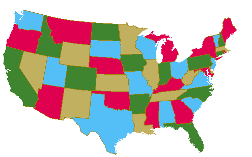
with at most four colors. Below is a map of the United State
colored using four colors

In graph terminology, this means that using at most four colors,
any planar graph (a graph that can be drawn without any of its
edges crossing) can have its nodes colored such that no two
adjacent nodes have the same color. The map version of the
theorem uses faces in place of nodes, where any two faces are
adjacent if and only if they share a border (an edge). Note
that a single point like the four corner border between Utah,
Arizona, Colorado, and New Mexico is not considered a border for
our purposes.
Make sure you understand that any map can be considered a graph where the faces of the map becomes nodes of the graph. For example, the four states Utah, Arizona, Colorado, and New Mexico considered alone as a graph would look like this: (insert simple square). We will henceforth think of a map as a graph.
The four-color theorem was conjectured in 1852 and proved in 1976
by Wolfgang Haken and Kenneth Appel at the University of Illinois
with the aid of a computer program that was thousands of lines
long and took over 1200 hours to run. Since that time, a
collective effort by interested mathematicians has been under way
to check the program. So far the only errors that have been found
are minor and were easily fixed. Many mathematicians accept the
theorem as true. There are many sites that summarize the
history and details of the problem.
Perhaps the most interesting feature of the 1976 proof is that it made use of a computer program to examine thousands of cases. This was at the time, and still is to some extent, a controversial and unprecedented use of computers in the actual proof of a theorem. The computer acted not merely as a tool for exploration, or as a way to implement a theory, but instead as a fundamental part of the fabric of the proof. Although the mathematics community accepted the correctness of the proof, there were and are still are those who question the proof's validity on philosophical grounds. "What makes a proof a proof?" they ask. Practically speaking, it is the confidence that competent mathematicians have checked the logic and meticulously scrutinized the details. But in this proof, the collective effort of hundreds of mathematicians for dozens of years would be necessary to check each case that the computer checked in a few hours. Even if such an effort were possible, it is hardly a feeling of confidence to know that any small error by anyone of hundreds of people would render the proof incorrect. If it is not practical then to cut the computer out of the picture, then how do we know for sure that the computer program is correct. Perhaps we could get mathematicians to formally check the correctness of the program, but how would we know for sure that the program ran correctly with certainty. It would not do to say that we are 99.999% sure the proof is correct. In math, a correct proof means 100%. These are some of the issues people have with this proof. Still the proof is accepted by the mathematical community at large, although even those who have no objection to its correctness, long for a more human elegant proof.
Ironically, a very elegant "proof" of the four color theorem was
"published" by Kempe
in 1879. The proof underwent the usual scrutiny of experts
and was published in a respectable journal. Eleven
years later Heawood
published a paper pointing out a flaw! This rare occurrence
of a refereed journal article with a proof containing a
serious logical error foreshadowed the even stranger results of
the 1975 computer aided proof. It happens often enough that
a journal referee will find errors in proofs, but often these
errors are easily corrected by the author. The rare times
when the errors are so serious that the author is unable to
correct them are almost always caught before the paper goes to
press. It was not so with Kempe's proof. You may be
wondering what kind of clever subtle unfixable flaw lurked in
Kempe's proof? You will soon find out. Perhaps you
will find the flaw yourself before it is pointed out
explicitly.
Luckily, Heawood was able to salvage some good results from the remains of Kempe's work. A number of excellent techniques remained as tools. And, with the flawed section removed, the remaining arguments correctly prove that five colors suffice.
In this lab, we study Kempe's proof and do some programming
experiments to explore his methods, and see if they can be used as
a (probabilistic or approximation) coloring algorithm. A
probabilistic algorithm is one that gets the correct aswer most of
the time; an approximation algorithm is one that gets close
to the correct answer every time. Irony is again the theme
here, as the algorithms based on Kempe's theory will work in
practice but defy a rigorous analysis. We have a proof that
is accomplished only with the help of a computer, and an algorithm
that seems to work even though it is based on a wrong proof!
This is truly a case study of the relationship between computer
science and mathematics.
Kempe's proof is constructive in the sense that the details of the proof imply a recursive algorithm for coloring. Kempe's proof is by induction on the number of regions in the map (or nodes in the graph). Like many difficult inductive proofs, he uses strong induction. This means he attempts to show that a graph with n nodes can be four-colored and assumes that all graphs with fewer than n nodes can be four-colored. This style is in mild contrast to the simple inductive proofs that we use for formulae like: 1+ 2+ 3 + ... + n = n(n+1)/2 where we start with nth case and work toward the n+1st case.
Before he gets to the inductive idea, Kempe begins with a clever way to categorize the possible graphs. He first states that we might as well consider graphs all of whose faces are triangles. These maximal planar graphs include the maximum number of edges possible, and if they can be four-colored, then so can other graphs with fewer edges. He then proves a lemma (a helper theorem) that any maximal planar graph must have at least one node with degree 5 or less. The proof uses Euler's Theorem for planar graphs and a counting argument to show that if all the nodes had degree 6 or higher, then the graph would not be planar. The details can be found below but they are not relevant to the main thread of the proof, and can be read independently.
If we denote the number of nodes,
edges, and faces (i.e., the bounded regions) of a planar graph by
V, E, and F respectively, then Euler's theorem for a plane (or a
sphere) is V - E + F = 2 (the outside
face counts too). Each face of a maximal planar graph is
bounded by three edges, and each edge is on the boundary of two
faces, so we have F = 2E/3. Euler's formula for a complete
planar graph then becomes simply E = 3V -
6. The degree of a
node is the number of edges incident to it. Now each edge is
connected to two nodes, so the sum of the degrees of all the nodes
2E = 6V - 12, and hence
the average degree per node is 6 -
12/V < 6, (assuming the graph is finite). This
implies that at least one vertex has degree five or less.
Exercise 1: Prove
Euler's theorem (thereby completing the proof above that in a
planar graph at least one vertex has degree five or less).
Your proof should use strong induction on the number of faces in
the graph. You can find this proof in many places. If
you can not figure it out on your own, then at least write it up
in your own words, showing clearly that you understand it!
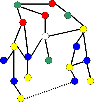
Figure 1 - A Simple Example
of a Kempe Chain. The B and Y nodes on the left side of
the graph are toggled, allowing x to be colored B.
Case 2: The subgraph includes the node adjacent to x colored Y. This is called a cyclical Kempe Chain. Now Kempe's idea does not work because the two nodes adjacent to x colored B and Y simply switch colors, and x is still adjacent to four different colors. Kempe fixes the problem by pointing out that if there is a path between the nodes adjacent to x colored B and Y, then there cannot be a path between the nodes colored G and R. The existence of one cyclical Kempe chain rules out the other, because one acts as a "barrier" between the nodes of the other. See Figure 2 below to see why.
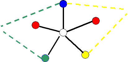
Figure 2 - Cyclical Kempe
Chains. One of the two Kempe chains, either B-Y or R-G,
is guaranteed not be cyclical
If there is no path between the nodes colored R or G, then
instead of creating the Kempe chain starting from the node
colored B, we start it
from R. That is,
create a subgraph by following the edges from R through all
nodes colored R or G. Then we can toggle the colors
R and G in this subgraph, and x
ends up adjacent to three colors: B, Y, and G. See figure
3 below.

Note that so far, Kempe's proof has no flaws.
Degree = 5
Figure 4 - The Two Cases for Degree 5. Case
1 is on the left and Case 2 on the right.
Case 1 is easy to handle, and the argument is similar to the degree 4 situation. The details are left as an exercise. The second case is the climax of Kempe's proof.
Exercise 2. Complete
the proof for Case 1 of Figure 4.

Figure 5 - The Hard Case. The B-Y and B-G chains are
rejected. Two new chains, one from each R node are used.
The R node on the right is recolored G, and R node on the left is
recolored Y, leaving R free for the center node x.
Exercise 3. Note that in Kempe's proof, when x is deleted from the graph, the resulting graph need not be connected. Look up the definition of strong induction. Explain why this implies that Kempe's proof uses strong mathematical induction.
The flaw in Kempe's proof, found by Heawood, is in the last
option of case 2 when the degree of x is 5, as he explains
the two Kempe chains emanating from the two red nodes as shown in
Figure 5. The problem is with the two sentences
below.
"The new Kempe chain with colors R and G cannot reach the node
adjacent to x colored
G, so the colors can be toggled and R becomes G. The new
Kempe chain with colors R and Y cannot reach the node adjacent to
x colored Y, so R
becomes Y."
The claim explains correctly why we can color all the nodes
adjacent to x without
using R, but there is an unexpected problem. It is possible
to have edges between Y nodes in the R-Y Kempe chain and G nodes
in the R-G Kempe chain! See the Y and G nodes at the top of
Figure 6.
Figure 6 - The Flaw
If we change the colors according to Kempe's methods, then both Y
and G both get changed to R! Without loss of generality,
assume Y is changed to R first. Then when G is changed To R
later, the Y, which is now R, gets changed to G, and that G may
have an edge to another G in the B-G Kempe subgraph.
Figure 5 misleads us into thinking that the G nodes surrounded by
the B-Y chain cannot be adjacent to any Y nodes surrounded by the
B-G chain, but they can! There it is in Figure 6. It
is helpful to try and convince yourself that this weird situation
cannot occur in the degree 4 argument, and that Figure 3 is not
similarly misleading.
Here is what John
Conway, a famous and flamboyant mathematician, and the
inventor of the game Life, has to say
about Kempe's proof and the flaw:
"I did read a few of the papers from this period, including Kempe's proof, Tait's deduction of his edge-coloring criterion from it, and an article in which Heawood pointed out the mistake, among other things, and the impression I got from them was much the same as Jim's. There was indeed a fair amount of interest in Kempe's "theorem", but not much evidence that any great number of people actually scrutinized his proof, or even read it. I don't think it would have made much difference if they had. The proof is very convincing, and in the days when the amateur provers were still interested in FCT, 2 times out of 3 "Kempe's Catastrophe", as Tom O'Beirne used to call it, was the proof they'd produce. Tom had a set lecture in which he gave Kempe's proof, illustrated by a specially made-up board with colored pegs, and seldom could anyone in the audience find anything wrong with it."
A fun paper
by Stan Wagon has a colored picture of the famous Errera
graph
on page 4. The Errera graph is a complete example
of a graph and coloring for which Kempe's proof fails.
One thing to notice is that the flaw requires quite a contrived
example, and in practice we may not see this happen very
often. In fact, the same graph but with a different coloring
might not reveal the flaw!
Create a four coloring algorithm based on Kempe's flawed proof. Your algorithm may fail due to the flaw in Kempe's proof, but it will always succeed in 5-coloring the graph, just as Kempe's proof is a correct 5-color proof.
Your algorithm should find a node of degree less than six, delete it from the graph, and recursively color the remainder of the graph. In the flawed case when the degree = 5, your algorithm will go ahead and build the Kempe chains, as Kempe described in his proof, hoping that it gets lucky and that the the flaw will not show up. If the flaw does show up, your algorithm will not be able to continue its four-coloring legally. You must check to see if this happens, and if it does, you can simply add a fifth color to color the deleted node. Kempe's flawed method never fails to five-color a graph.
The details of this algorithm are not simple, but they are
standard. You need to use a graph data structure, either an
adjacency matrix or an array of adjacency linked lists. The
algorithm works recursively, by searching for any node of degree
less than six, and deleting it from the graph. The resulting
graph (or graphs - the pieces may not all be connected)
is/are colored recursively. You algorithm needs to then
color the node it deleted making sure it uses one of the four
colors used by the recursive coloring. The cases are exactly
like those in Kempe's proof.
There is one technical issue that you probably won't think of on your own, that comes up in the case of a deleted node of degree 4 or 5. Consider the degree 4 case. When you have the adjacent colors B, G, Y, and R. With Kempe's picture, it is clear which nodes are opposite each other. B is opposite Y, and G is opposite R. In this case as we described earlier, you do a depth first search from B looking for colors B and Y, and if necessary, another depth first search from R looking for colors R and G. In the end, you have a free color for the deleted node that you are trying to color. However, in a regular graph data structure it is not at all obvious which nodes are "opposite" each other. That is, we have no way to know which nodes share a face, because we have no special data structure for the details of the planar embedding. Hence if you started a depth first search from a node with a particular color, you would not know which other color to search for.
The easiest way to handle this without opening a Pandora's box of data structures, is to
The case for degree 5 is similar, and you will need to try all 4 possible nodes as opposite. Of course the flaw is in the degree 5 case, so if none of them of the 4 possibilities work, you add a fifth color as described earlier.
You should experiment with your algorithm and see if it ever
fails. Use the graph of the map of the USA which you can
find here.
Exercise 5. What is
the complexity of your Kempe-based algorithm? Explain your
analysis.
Note, there is a quadratic
time
algorithm to 4-color a planar graph, but it uses techniques
from a correct proof that are too hard for us to consider
here. Is your pseudo-correct algorithm faster or slower than
this one?